<?xml version="1.0" encoding="UTF-8"?><feed xmlns="http://www.w3.org/2005/Atom"><link type="application/atom+xml" title="blip.kummerlaender.eu" rel="self" href="https://blip.kummerlaender.eu/atom.xml"/><id>https://blip.kummerlaender.eu/atom.xml</id><title>Latest commits @ blip.kummerlaender.eu</title><updated>2025_08_25T20:03:00+02:00</updated><entry><id>https://doi.org/10.1016/j.jpdc.2025.105169</id><title>Optimizing LBM performance on heterogeneous CPU-GPU systems</title><link title="Optimizing LBM performance on heterogeneous CPU-GPU systems" rel="alternate" href="https://doi.org/10.1016/j.jpdc.2025.105169"/><author><name>Adrian Kummerländer</name></author><updated>2025_08_25T20:03:00+02:00</updated><content type="xhtml"><div xmlns="http://www.w3.org/1999/xhtml"><p>The full paper of the work I presented way back in 2023 at the DSFD in Albuquerque has been accepted by the <em>Journal of Parallel and Distributed Computing</em> after initial submission in January 2024. Things in OpenLB have improved even more since then and my paper draft pipeline is… overwhelming. Still, it is very nice to finally see this published.</p><p>The main result is that up to 1.8-fold speedups can be obtained for various LES simulation cases by switching to a cooperative CPU-GPU load balancing strategy from pure GPU-only execution. Different from similar approaches, the underyling domain decomposition is optimized from bottom up to be suited to heterogeneous execution using a genetic algorithm. A detailed description of this methodology is backed by extensive performance evaluations and timing profiles.</p></div></content></entry><entry><id>https://www.lbrg.kit.edu/~akummerlaender/</id><title>Publications and talks</title><link title="Publications and talks" rel="alternate" href="https://www.lbrg.kit.edu/~akummerlaender/"/><author><name>Adrian Kummerländer</name></author><updated>2022_10_24T11:12:00+02:00</updated><content type="xhtml"><div xmlns="http://www.w3.org/1999/xhtml"><p>Today my first paper on implicit propagation in directly addressed grids was accepted for publication in <a href="https://onlinelibrary.wiley.com/journal/15320634">Concurrency and Computation</a>. It will soon be available as open access under DOI <code>10.1002/cpe.7509</code>.</p><p>In other news, the annual report of our cluster usage <em>Advances in Computational Process Engineering using Lattice Boltzmann Methods on High Performance Computers for Solving Fluid Flow Problems</em> was accepted for publication in the annual proceedings on <em>High Performance Computing in Science and Engineering</em> by the <a href="https://www.hlrs.de/">High Performance Computing Center Stuttgart (HLRS)</a>. In this context I was also offered the opportunity of presenting it in person at the <a href="https://www.hlrs.de/event/2022/review-ws-25">25th Results and Review Workshop</a>.</p><p>If you are interested in more details along those lines, I will give a talk on <em>Lattice Boltzmann Performance Engineering in OpenLB</em> at the Helmholtz <a href="https://www.helmholtz-hirse.de/events/2022_12_01-seminar_9.html">HiRSE seminar</a> on December 1st.</p></div></content></entry><entry><id>https://www.openlb.net/news/openlb-release-1-5-available-for-download/</id><title>Released OpenLB 1.5</title><link title="Released OpenLB 1.5" rel="alternate" href="https://www.openlb.net/news/openlb-release-1-5-available-for-download/"/><author><name>Adrian Kummerländer</name></author><updated>2022_04_14T12:00:00+02:00</updated><content type="xhtml"><div xmlns="http://www.w3.org/1999/xhtml"><p>Today <a href="https://www.lbrg.kit.edu/">we</a> released OpenLB 1.5 which marks a major step forwards by including both support for usage of GPUs and for vectorization on CPUs. These performance focused improvements are the result of major refactoring efforts that spanned both a significant fraction of my time as a student and most of my first months as a doctoral student.</p><p>For some further information check out the <a href="https://www.openlb.net/performance/">performance section</a> of the OpenLB website. <a href="https://www.youtube.com/watch?v=vprFLUMwik0">A recent video</a> augments this by some pretty visuals produced on <a href="https://www.scc.kit.edu/en/services/horeka.php">HoreKa’s</a> GPU partition.</p></div></content></entry><entry><id>http://dx.doi.org/10.13140/RG.2.2.35085.87523</id><title>Submitted my first paper</title><link title="Submitted my first paper" rel="alternate" href="http://dx.doi.org/10.13140/RG.2.2.35085.87523"/><author><name>Adrian Kummerländer</name></author><updated>2021_08_04T15:30:00+02:00</updated><content type="xhtml"><div xmlns="http://www.w3.org/1999/xhtml"><p>Today I submitted the full paper of my talk at the <a href="https://parcfd2020.sciencesconf.org/">32nd ParCFD</a> conference for publication.</p><p>There we consider the LBM algorithm’s propagation step as a transformation of the space filling curve used as the memory bijection. Specifically, a neighborhood distance invariance property is utilized to derive the existing <em>Shift-Swap-Streaming (SSS)</em> scheme as well as a new <em>Periodic Shift (PS)</em> pattern.</p><p>A special focus is placed on SIMD friendly implementation via virtual memory mapping on both CPU and GPU targets.</p><p>Both patterns are evaluated in detailed benchmarks. PS is found to provide consistent bandwidth-related performance while imposing minimal restrictions on the collision implementation.</p><p>The preprint is available on <a href="http://dx.doi.org/10.13140/RG.2.2.35085.87523">Researchgate</a> as well as <a href="https://static.kummerlaender.eu/media/preprint_implicit_propagation.pdf">directly (PDF)</a>.</p></div></content></entry><entry><id>https://tree.kummerlaender.eu/projects/math/md_benzene</id><title>Molecular Dynamics Simulation of the Benzene Dimer</title><link title="Molecular Dynamics Simulation of the Benzene Dimer" rel="alternate" href="https://tree.kummerlaender.eu/projects/math/md_benzene"/><author><name>Adrian Kummerländer</name></author><updated>2021_03_31T20:05:00+02:00</updated><content type="xhtml"><div xmlns="http://www.w3.org/1999/xhtml"><p>
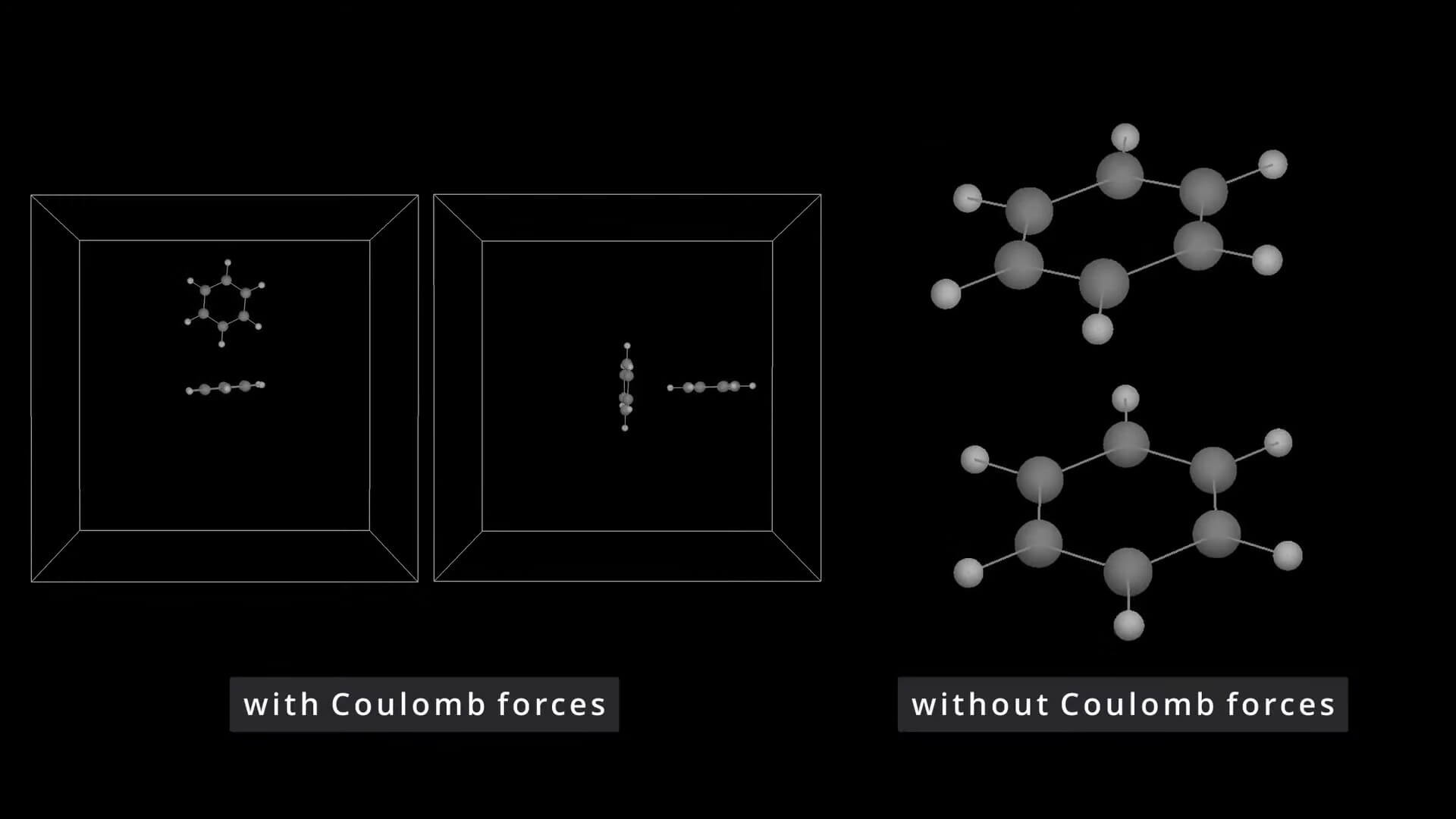
One of the last lectures for my master’s degree was on numerical simulation in molecular dynamics. For the <a href="https://tree.kummerlaender.eu/projects/math/md_benzene">examination project</a> I developed a <a href="https://tree.kummerlaender.eu/projects/interacticle">GPU MD code</a> capable of reproducing certain preferred configurations the benzene dimer.
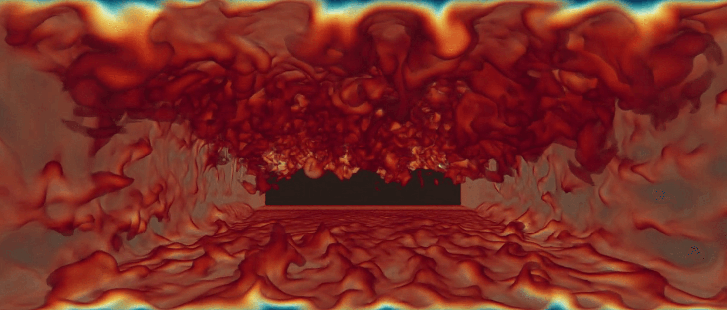
</p><p><a href="https://youtu.be/8pNgH4Rt9eo"><img src="https://static.kummerlaender.eu/media/md_benzene_teaser.jpg"/></a></p></div></content></entry><entry><id>https://www.youtube.com/watch?v=J2al5tV14M8&amp;list=PLRqmRhcPBBPscHlIRCMnN3vdocqoC8OLD</id><title>Just-in-time volumetric CFD visualization</title><link title="Just-in-time volumetric CFD visualization" rel="alternate" href="https://www.youtube.com/watch?v=J2al5tV14M8&amp;list=PLRqmRhcPBBPscHlIRCMnN3vdocqoC8OLD"/><author><name>Adrian Kummerländer</name></author><updated>2020_07_24T14:15:00+02:00</updated><content type="xhtml"><div xmlns="http://www.w3.org/1999/xhtml"><p>For my <a href="https://literatelb.org/talk/">seminar talk</a> I wrote another LBM solver as a literate Org-document using CUDA and SymPy. The main focus was on just-in-time volumetric visualizations of the simulations performed by this code. While this is not ready to publish yet, check out the following impressions:
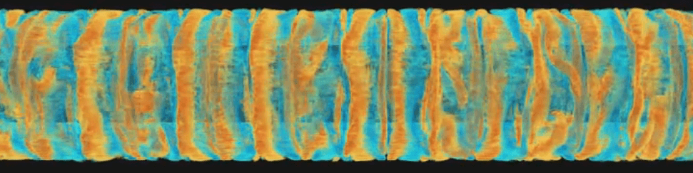
</p><p><a href="https://www.youtube.com/watch?v=B-LKZPWM0S0"><img alt="Flow around a rotating shaft" src="https://static.kummerlaender.eu/media/llbm_preview_1.png"/></a></p><p>Further videos are available on my <a href="https://www.youtube.com/watch?v=B-LKZPWM0S0">YouTube channel</a>. e.g. a Taylor-Couette flow:</p><p><a href="https://www.youtube.com/watch?v=xEENH4sZBDQ"><img alt="Taylor-Couette flow" src="https://static.kummerlaender.eu/media/llbm_preview_2.png"/></a></p></div></content></entry><entry><id>https://www.youtube.com/watch?v=ITJ1j78k1eM</id><title>Visualizing the velocity distribution of a hard sphere gas</title><link title="Visualizing the velocity distribution of a hard sphere gas" rel="alternate" href="https://www.youtube.com/watch?v=ITJ1j78k1eM"/><author><name>Adrian Kummerländer</name></author><updated>2020_03_24T21:42:00+02:00</updated><content type="xhtml"><div xmlns="http://www.w3.org/1999/xhtml"><p>
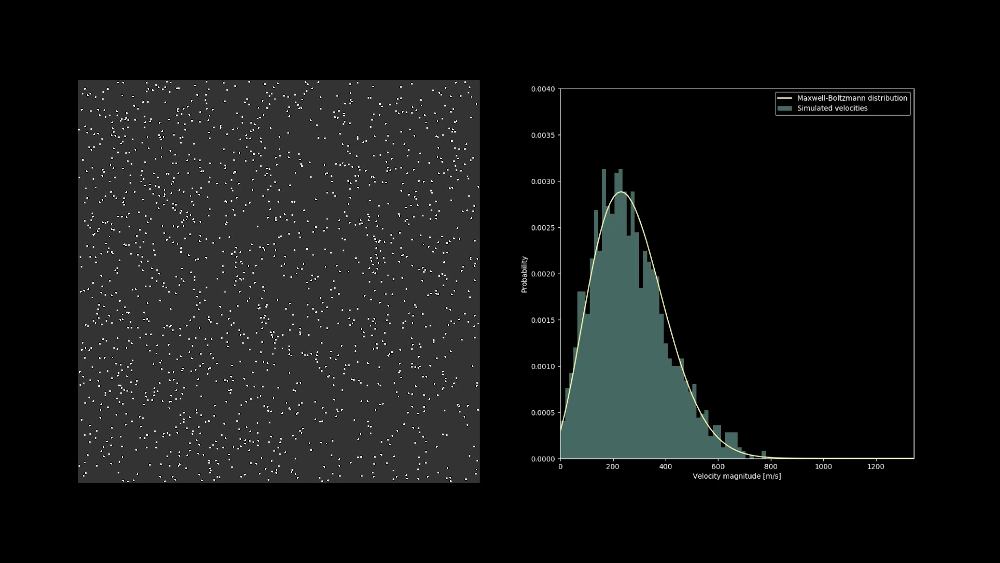
The velocity distribution of a system of colliding hard sphere particles quickly evolves into the Maxwell-Boltzmann distribution. One example of this surprisingly quick process can be seen in the following video:</p><p><a href="https://www.youtube.com/watch?v=ITJ1j78k1eM"><img alt="Simulation of hard sphere gas" src="https://static.kummerlaender.eu/media/boltzgas_teaser.png"/></a></p></div></content></entry><entry><id>https://code.kummerlaender.eu/firmament/commit/?id=071bc3e6439d7775e9684dfeeb27d423d47167a9</id><title>Visualize the sky for arbitrary time and space coordinates on earth</title><link title="Visualize the sky for arbitrary time and space coordinates on earth" rel="alternate" href="https://code.kummerlaender.eu/firmament/commit/?id=071bc3e6439d7775e9684dfeeb27d423d47167a9"/><author><name>Adrian Kummerländer</name></author><updated>2020_01_11T21:12:00+02:00</updated><content type="xhtml"><div xmlns="http://www.w3.org/1999/xhtml"><p>The primary color of the sky is caused by Rayleigh and Mie scattering of light in the atmosphere. While attending the lecture on <a href="http://www.math.kit.edu/ianm2/edu/mathmodelsim2019w/de">Mathematical Modelling and Simulation</a> at KIT I implemented a ray marcher to visualize this. Together with a model for calculating the sun direction for given coordinates and times this allows for generating interesting plots:</p><p><a href="https://www.youtube.com/watch?v=aewYpD883WY"><img alt="Sky in August" src="https://code.kummerlaender.eu/firmament/plain/example/2020-08-01_12-00-00_firmament_at_karlsruhe_palace.png"/></a></p><p>For more details check out <a href="https://tree.kummerlaender.eu/projects/firmament/">Firmament</a>.</p></div></content></entry><entry><id>https://github.com/KnairdA/boltzgen</id><title>Started working on a framework for generating LBM kernels</title><link title="Started working on a framework for generating LBM kernels" rel="alternate" href="https://github.com/KnairdA/boltzgen"/><author><name>Adrian Kummerländer</name></author><updated>2019_10_27T22:35:00+02:00</updated><content type="xhtml"><div xmlns="http://www.w3.org/1999/xhtml"><p>During the past exam season I now and then continued to play around with my GPU LBM code <a href="https://tree.kummerlaender.eu/projects/symlbm_playground/">symlbm_playground</a>. While I mostly focused on generating various real-time visualizations using e.g. volumetric ray marching, the underlying principle of generating OpenCL kernels from a symbolic description has not lost its promise.</p><p>This is why I have now started to extract the generator part of this past project into a more general framework. Currently <a href="https://code.kummerlaender.eu/boltzgen/about/">boltzgen</a> targets C++ and OpenCL using a shared symbolic description while providing various configuration options:</p><pre>λ ~<span style="color:#f8f8f2">/</span>p<span style="color:#f8f8f2">/</span>d<span style="color:#f8f8f2">/</span>boltzgen <span style="color:#f8f8f2">(</span>boltzgen<span style="color:#66d9ef">-env</span><span style="color:#f8f8f2">)</span> ● .<span style="color:#f8f8f2">/</span>boltzgen.py <span style="color:#66d9ef">--help</span>
usage<span style="color:#f8f8f2">:</span> boltzgen.py <span style="color:#f8f8f2">[</span><span style="color:#66d9ef">-h</span><span style="color:#f8f8f2">]</span> <span style="color:#66d9ef">--lattice</span> LATTICE <span style="color:#66d9ef">--layout</span> LAYOUT <span style="color:#66d9ef">--precision</span>
                   PRECISION <span style="color:#66d9ef">--geometry</span> GEOMETRY <span style="color:#66d9ef">--tau</span> TAU <span style="color:#f8f8f2">[</span><span style="color:#66d9ef">--disable-cse</span><span style="color:#f8f8f2">]</span>
                   <span style="color:#f8f8f2">[</span><span style="color:#66d9ef">--functions</span> FUNCTIONS <span style="color:#f8f8f2">[</span>FUNCTIONS ...<span style="color:#f8f8f2">]]</span>
                   <span style="color:#f8f8f2">[</span><span style="color:#66d9ef">--extras</span> EXTRAS <span style="color:#f8f8f2">[</span>EXTRAS ...<span style="color:#f8f8f2">]]</span>
                   language

Generate LBM kernels <span style="color:#f92672; font-weight:bold">in</span> various languages using a symbolic description.

positional arguments<span style="color:#f8f8f2">:</span>
  language              Target language <span style="color:#f8f8f2">(</span>currently either <span style="color:#e6db74">"cl"</span> or <span style="color:#e6db74">"cpp"</span><span style="color:#f8f8f2">)</span>

optional arguments<span style="color:#f8f8f2">:</span>
  <span style="color:#66d9ef">-h</span><span style="color:#f8f8f2">,</span> <span style="color:#66d9ef">--help</span>            show this <span style="color:#66d9ef">help</span> message and <span style="color:#66d9ef">exit</span>
  <span style="color:#66d9ef">--lattice</span> LATTICE     Lattice <span style="color:#66d9ef">type</span> <span style="color:#f8f8f2">(</span>D2Q9<span style="color:#f8f8f2">,</span> D3Q7<span style="color:#f8f8f2">,</span> D3Q19<span style="color:#f8f8f2">,</span> D3Q27<span style="color:#f8f8f2">)</span>
  <span style="color:#66d9ef">--layout</span> LAYOUT       Memory layout <span style="color:#f8f8f2">(</span><span style="color:#e6db74">"AOS"</span> or <span style="color:#e6db74">"SOA"</span><span style="color:#f8f8f2">)</span>
  <span style="color:#66d9ef">--precision</span> PRECISION
                        Floating precision <span style="color:#f8f8f2">(</span><span style="color:#e6db74">"single"</span> or <span style="color:#e6db74">"double"</span><span style="color:#f8f8f2">)</span>
  <span style="color:#66d9ef">--geometry</span> GEOMETRY   Size of the block geometry <span style="color:#f8f8f2">(</span><span style="color:#e6db74">"x:y(:z)"</span><span style="color:#f8f8f2">)</span>
  <span style="color:#66d9ef">--tau</span> TAU             BGK relaxation <span style="color:#f92672; font-weight:bold">time</span>
  <span style="color:#66d9ef">--disable-cse</span>         Disable common subexpression elimination
  <span style="color:#66d9ef">--functions</span> FUNCTIONS <span style="color:#f8f8f2">[</span>FUNCTIONS ...<span style="color:#f8f8f2">]</span>
                        Function templates to be generated
  <span style="color:#66d9ef">--extras</span> EXTRAS <span style="color:#f8f8f2">[</span>EXTRAS ...<span style="color:#f8f8f2">]</span>
                        Additional generator parameters
</pre><p>The goal is to build upon this foundation to provide an easy way to generate efficient code using a high level description of various collision models and boundary conditions. This should allow for easy comparision between various streaming patterns and memory layouts.</p></div></content></entry><entry><id>https://code.kummerlaender.eu/symlbm_playground/commit/?id=d71faec93ec0a55c46810e0d178b2803ee89130c</id><title>Symbolically generate D3Q19 OpenCL kernel using SymPy</title><link title="Symbolically generate D3Q19 OpenCL kernel using SymPy" rel="alternate" href="https://code.kummerlaender.eu/symlbm_playground/commit/?id=d71faec93ec0a55c46810e0d178b2803ee89130c"/><author><name>Adrian Kummerländer</name></author><updated>2019_06_15T20:45:00+02:00</updated><content type="xhtml"><div xmlns="http://www.w3.org/1999/xhtml"><p>My recent experiments in using the <a href="https://www.sympy.org/">SymPy</a> CAS library for automatically deriving optimized LBM codes have now evolved to the point where a single generator produces both D2Q9 and D3Q19 OpenCL kernels.</p><video controls="" loop="true" poster="https://static.kummerlaender.eu/media/ldc_3d.poster.jpg" preload="metadata" style="max-width:100%">
<source src="https://static.kummerlaender.eu/media/ldc_3d.mp4" type="video/mp4"/>
</video><p>Automatically deriving kernel implementations from the symbolic formulation of e.g. the BGK relaxation operator presents itself as a very powerful concept. This could potentially be developed to the point where a LBM specific code generator could produce highly optimized GPU programs tailored to arbitrary simulation problems.</p></div></content></entry><entry><id>https://code.kummerlaender.eu/compustream/commit/?id=ecaf665a05bdfcd10937152c378cfaec7cdf1836</id><title>Experimental visualization of the velocity curl</title><link title="Experimental visualization of the velocity curl" rel="alternate" href="https://code.kummerlaender.eu/compustream/commit/?id=ecaf665a05bdfcd10937152c378cfaec7cdf1836"/><author><name>Adrian Kummerländer</name></author><updated>2019_04_28T12:53:00+02:00</updated><content type="xhtml"><div xmlns="http://www.w3.org/1999/xhtml"><p>Calculating the curl of our simulated velocity field requires an additional compute shader step. Handling of buffer and shader switching depending on the display mode is implemented rudimentarily for now. Most of this commit is scaffolding, the actual computation is more or less trivial:</p><pre><span style="color:#66d9ef">const float</span> dxvy <span style="color:#f8f8f2">= (</span><span style="color:#25faac">getFluidVelocity</span><span style="color:#f8f8f2">(</span>x<span style="color:#f8f8f2">+</span><span style="color:#ae81ff">1</span><span style="color:#f8f8f2">,</span>y<span style="color:#f8f8f2">).</span>y <span style="color:#f8f8f2">-</span> <span style="color:#25faac">getFluidVelocity</span><span style="color:#f8f8f2">(</span>x<span style="color:#f8f8f2">-</span><span style="color:#ae81ff">1</span><span style="color:#f8f8f2">,</span>y<span style="color:#f8f8f2">).</span>y<span style="color:#f8f8f2">)</span>
                 <span style="color:#f8f8f2">/ (</span><span style="color:#ae81ff">2</span><span style="color:#f8f8f2">*</span>convLength<span style="color:#f8f8f2">);</span>
<span style="color:#66d9ef">const float</span> dyvx <span style="color:#f8f8f2">= (</span><span style="color:#25faac">getFluidVelocity</span><span style="color:#f8f8f2">(</span>x<span style="color:#f8f8f2">,</span>y<span style="color:#f8f8f2">+</span><span style="color:#ae81ff">1</span><span style="color:#f8f8f2">).</span>x <span style="color:#f8f8f2">-</span> <span style="color:#25faac">getFluidVelocity</span><span style="color:#f8f8f2">(</span>x<span style="color:#f8f8f2">,</span>y<span style="color:#f8f8f2">-</span><span style="color:#ae81ff">1</span><span style="color:#f8f8f2">).</span>x<span style="color:#f8f8f2">)</span>
                 <span style="color:#f8f8f2">/ (</span><span style="color:#ae81ff">2</span><span style="color:#f8f8f2">*</span>convLength<span style="color:#f8f8f2">);</span>

<span style="color:#25faac">setFluidExtra</span><span style="color:#f8f8f2">(</span>x<span style="color:#f8f8f2">,</span> y<span style="color:#f8f8f2">,</span> dxvy <span style="color:#f8f8f2">-</span> dyvx<span style="color:#f8f8f2">);</span>
</pre><p>This implements the following discretization of the 2d curl operator:</p><p>Let <span class="math"><span class="katex"><span class="katex-mathml"><math><semantics><mrow><mi>V</mi><mo>:</mo><msup><mi mathvariant="double-struck">N</mi><mn>2</mn></msup><mo>→</mo><msup><mi mathvariant="double-struck">R</mi><mn>2</mn></msup></mrow><annotation encoding="application/x-tex">V : \mathbb{N}^2 \to \mathbb{R}^2</annotation></semantics></math></span><span aria-hidden="true" class="katex-html"><span class="base"><span class="strut" style="height:0.68333em;vertical-align:0em;"><!----></span><span class="mord mathdefault" style="margin-right:0.22222em;">V</span><span class="mspace" style="margin-right:0.2777777777777778em;"><!----></span><span class="mrel">:</span><span class="mspace" style="margin-right:0.2777777777777778em;"><!----></span></span><span class="base"><span class="strut" style="height:0.8141079999999999em;vertical-align:0em;"><!----></span><span class="mord"><span class="mord"><span class="mord mathbb">N</span></span><span class="msupsub"><span class="vlist-t"><span class="vlist-r"><span class="vlist" style="height:0.8141079999999999em;"><span style="top:-3.063em;margin-right:0.05em;"><span class="pstrut" style="height:2.7em;"><!----></span><span class="sizing reset-size6 size3 mtight"><span class="mord mtight">2</span></span></span></span></span></span></span></span><span class="mspace" style="margin-right:0.2777777777777778em;"><!----></span><span class="mrel">→</span><span class="mspace" style="margin-right:0.2777777777777778em;"><!----></span></span><span class="base"><span class="strut" style="height:0.8141079999999999em;vertical-align:0em;"><!----></span><span class="mord"><span class="mord"><span class="mord mathbb">R</span></span><span class="msupsub"><span class="vlist-t"><span class="vlist-r"><span class="vlist" style="height:0.8141079999999999em;"><span style="top:-3.063em;margin-right:0.05em;"><span class="pstrut" style="height:2.7em;"><!----></span><span class="sizing reset-size6 size3 mtight"><span class="mord mtight">2</span></span></span></span></span></span></span></span></span></span></span></span> be the simulated velocity field at discrete lattice points spaced by <span class="math"><span class="katex"><span class="katex-mathml"><math><semantics><mrow><mi mathvariant="normal">Δ</mi><mi>x</mi><mo>∈</mo><msub><mi mathvariant="double-struck">R</mi><mrow><mo>&gt;</mo><mn>0</mn></mrow></msub></mrow><annotation encoding="application/x-tex">\Delta x \in \mathbb{R}_{\gt 0}</annotation></semantics></math></span><span aria-hidden="true" class="katex-html"><span class="base"><span class="strut" style="height:0.72243em;vertical-align:-0.0391em;"><!----></span><span class="mord">Δ</span><span class="mord mathdefault">x</span><span class="mspace" style="margin-right:0.2777777777777778em;"><!----></span><span class="mrel">∈</span><span class="mspace" style="margin-right:0.2777777777777778em;"><!----></span></span><span class="base"><span class="strut" style="height:0.86626em;vertical-align:-0.17737em;"><!----></span><span class="mord"><span class="mord"><span class="mord mathbb">R</span></span><span class="msupsub"><span class="vlist-t vlist-t2"><span class="vlist-r"><span class="vlist" style="height:0.30110799999999993em;"><span style="top:-2.5500000000000003em;margin-right:0.05em;"><span class="pstrut" style="height:2.7em;"><!----></span><span class="sizing reset-size6 size3 mtight"><span class="mord mtight"><span class="mrel mtight">&gt;</span><span class="mord mtight">0</span></span></span></span></span><span class="vlist-s">​</span></span><span class="vlist-r"><span class="vlist" style="height:0.17737em;"><span><!----></span></span></span></span></span></span></span></span></span></span>. We want to approximate the <span class="math"><span class="katex"><span class="katex-mathml"><math><semantics><mrow><mi>z</mi></mrow><annotation encoding="application/x-tex">z</annotation></semantics></math></span><span aria-hidden="true" class="katex-html"><span class="base"><span class="strut" style="height:0.43056em;vertical-align:0em;"><!----></span><span class="mord mathdefault" style="margin-right:0.04398em;">z</span></span></span></span></span>-component of the curl for visualization: <p class="math"><span class="katex-display"><span class="katex"><span class="katex-mathml"><math><semantics><mrow><mi>ω</mi><mo>:</mo><mo>=</mo><msub><mi mathvariant="normal">∂</mi><mi>x</mi></msub><msub><mi>V</mi><mi>y</mi></msub><mo>−</mo><msub><mi mathvariant="normal">∂</mi><mi>y</mi></msub><msub><mi>V</mi><mi>x</mi></msub></mrow><annotation encoding="application/x-tex">\omega := \partial_x V_y - \partial_y V_x</annotation></semantics></math></span><span aria-hidden="true" class="katex-html"><span class="base"><span class="strut" style="height:0.43056em;vertical-align:0em;"><!----></span><span class="mord mathdefault" style="margin-right:0.03588em;">ω</span><span class="mspace" style="margin-right:0.2777777777777778em;"><!----></span><span class="mrel">:</span></span><span class="base"><span class="strut" style="height:0.36687em;vertical-align:0em;"><!----></span><span class="mrel">=</span><span class="mspace" style="margin-right:0.2777777777777778em;"><!----></span></span><span class="base"><span class="strut" style="height:0.980548em;vertical-align:-0.286108em;"><!----></span><span class="mord"><span class="mord" style="margin-right:0.05556em;">∂</span><span class="msupsub"><span class="vlist-t vlist-t2"><span class="vlist-r"><span class="vlist" style="height:0.151392em;"><span style="top:-2.5500000000000003em;margin-left:-0.05556em;margin-right:0.05em;"><span class="pstrut" style="height:2.7em;"><!----></span><span class="sizing reset-size6 size3 mtight"><span class="mord mathdefault mtight">x</span></span></span></span><span class="vlist-s">​</span></span><span class="vlist-r"><span class="vlist" style="height:0.15em;"><span><!----></span></span></span></span></span></span><span class="mord"><span class="mord mathdefault" style="margin-right:0.22222em;">V</span><span class="msupsub"><span class="vlist-t vlist-t2"><span class="vlist-r"><span class="vlist" style="height:0.15139200000000003em;"><span style="top:-2.5500000000000003em;margin-left:-0.22222em;margin-right:0.05em;"><span class="pstrut" style="height:2.7em;"><!----></span><span class="sizing reset-size6 size3 mtight"><span class="mord mathdefault mtight" style="margin-right:0.03588em;">y</span></span></span></span><span class="vlist-s">​</span></span><span class="vlist-r"><span class="vlist" style="height:0.286108em;"><span><!----></span></span></span></span></span></span><span class="mspace" style="margin-right:0.2222222222222222em;"><!----></span><span class="mbin">−</span><span class="mspace" style="margin-right:0.2222222222222222em;"><!----></span></span><span class="base"><span class="strut" style="height:0.980548em;vertical-align:-0.286108em;"><!----></span><span class="mord"><span class="mord" style="margin-right:0.05556em;">∂</span><span class="msupsub"><span class="vlist-t vlist-t2"><span class="vlist-r"><span class="vlist" style="height:0.15139200000000003em;"><span style="top:-2.5500000000000003em;margin-left:-0.05556em;margin-right:0.05em;"><span class="pstrut" style="height:2.7em;"><!----></span><span class="sizing reset-size6 size3 mtight"><span class="mord mathdefault mtight" style="margin-right:0.03588em;">y</span></span></span></span><span class="vlist-s">​</span></span><span class="vlist-r"><span class="vlist" style="height:0.286108em;"><span><!----></span></span></span></span></span></span><span class="mord"><span class="mord mathdefault" style="margin-right:0.22222em;">V</span><span class="msupsub"><span class="vlist-t vlist-t2"><span class="vlist-r"><span class="vlist" style="height:0.151392em;"><span style="top:-2.5500000000000003em;margin-left:-0.22222em;margin-right:0.05em;"><span class="pstrut" style="height:2.7em;"><!----></span><span class="sizing reset-size6 size3 mtight"><span class="mord mathdefault mtight">x</span></span></span></span><span class="vlist-s">​</span></span><span class="vlist-r"><span class="vlist" style="height:0.15em;"><span><!----></span></span></span></span></span></span></span></span></span></span></p></p><p>As we do not possess the actual function <span class="math"><span class="katex"><span class="katex-mathml"><math><semantics><mrow><mi>V</mi></mrow><annotation encoding="application/x-tex">V</annotation></semantics></math></span><span aria-hidden="true" class="katex-html"><span class="base"><span class="strut" style="height:0.68333em;vertical-align:0em;"><!----></span><span class="mord mathdefault" style="margin-right:0.22222em;">V</span></span></span></span></span> but only its values at a set of discrete points we approximate the two partial derivatives using a second order central difference scheme: <p class="math"><span class="katex-display"><span class="katex"><span class="katex-mathml"><math><semantics><mrow><mover accent="true"><mi>ω</mi><mo stretchy="true">‾</mo></mover><mo>(</mo><mi>i</mi><mo separator="true">,</mo><mi>j</mi><mo>)</mo><mo>:</mo><mo>=</mo><mfrac><mrow><msub><mi>V</mi><mi>y</mi></msub><mo>(</mo><mi>i</mi><mo>+</mo><mn>1</mn><mo separator="true">,</mo><mi>j</mi><mo>)</mo><mo>−</mo><msub><mi>V</mi><mi>y</mi></msub><mo>(</mo><mi>i</mi><mo>−</mo><mn>1</mn><mo separator="true">,</mo><mi>j</mi><mo>)</mo></mrow><mrow><mn>2</mn><mi mathvariant="normal">Δ</mi><mi>x</mi></mrow></mfrac><mo>−</mo><mfrac><mrow><msub><mi>V</mi><mi>x</mi></msub><mo>(</mo><mi>i</mi><mo separator="true">,</mo><mi>j</mi><mo>+</mo><mn>1</mn><mo>)</mo><mo>−</mo><msub><mi>V</mi><mi>x</mi></msub><mo>(</mo><mi>i</mi><mo separator="true">,</mo><mi>j</mi><mo>−</mo><mn>1</mn><mo>)</mo></mrow><mrow><mn>2</mn><mi mathvariant="normal">Δ</mi><mi>x</mi></mrow></mfrac></mrow><annotation encoding="application/x-tex">\overline{\omega}(i,j) := \frac{V_y(i+1,j) - V_y(i-1,j)}{2 \Delta x} - \frac{V_x(i,j+1) - V_x(i,j-1)}{2 \Delta x}</annotation></semantics></math></span><span aria-hidden="true" class="katex-html"><span class="base"><span class="strut" style="height:1em;vertical-align:-0.25em;"><!----></span><span class="mord overline"><span class="vlist-t"><span class="vlist-r"><span class="vlist" style="height:0.63056em;"><span style="top:-3em;"><span class="pstrut" style="height:3em;"><!----></span><span class="mord"><span class="mord mathdefault" style="margin-right:0.03588em;">ω</span></span></span><span style="top:-3.55056em;"><span class="pstrut" style="height:3em;"><!----></span><span class="overline-line" style="border-bottom-width:0.04em;"><!----></span></span></span></span></span></span><span class="mopen">(</span><span class="mord mathdefault">i</span><span class="mpunct">,</span><span class="mspace" style="margin-right:0.16666666666666666em;"><!----></span><span class="mord mathdefault" style="margin-right:0.05724em;">j</span><span class="mclose">)</span><span class="mspace" style="margin-right:0.2777777777777778em;"><!----></span><span class="mrel">:</span></span><span class="base"><span class="strut" style="height:0.36687em;vertical-align:0em;"><!----></span><span class="mrel">=</span><span class="mspace" style="margin-right:0.2777777777777778em;"><!----></span></span><span class="base"><span class="strut" style="height:2.113em;vertical-align:-0.686em;"><!----></span><span class="mord"><span class="mopen nulldelimiter"><!----></span><span class="mfrac"><span class="vlist-t vlist-t2"><span class="vlist-r"><span class="vlist" style="height:1.427em;"><span style="top:-2.314em;"><span class="pstrut" style="height:3em;"><!----></span><span class="mord"><span class="mord">2</span><span class="mord">Δ</span><span class="mord mathdefault">x</span></span></span><span style="top:-3.23em;"><span class="pstrut" style="height:3em;"><!----></span><span class="frac-line" style="border-bottom-width:0.04em;"><!----></span></span><span style="top:-3.677em;"><span class="pstrut" style="height:3em;"><!----></span><span class="mord"><span class="mord"><span class="mord mathdefault" style="margin-right:0.22222em;">V</span><span class="msupsub"><span class="vlist-t vlist-t2"><span class="vlist-r"><span class="vlist" style="height:0.15139200000000003em;"><span style="top:-2.5500000000000003em;margin-left:-0.22222em;margin-right:0.05em;"><span class="pstrut" style="height:2.7em;"><!----></span><span class="sizing reset-size6 size3 mtight"><span class="mord mathdefault mtight" style="margin-right:0.03588em;">y</span></span></span></span><span class="vlist-s">​</span></span><span class="vlist-r"><span class="vlist" style="height:0.286108em;"><span><!----></span></span></span></span></span></span><span class="mopen">(</span><span class="mord mathdefault">i</span><span class="mspace" style="margin-right:0.2222222222222222em;"><!----></span><span class="mbin">+</span><span class="mspace" style="margin-right:0.2222222222222222em;"><!----></span><span class="mord">1</span><span class="mpunct">,</span><span class="mspace" style="margin-right:0.16666666666666666em;"><!----></span><span class="mord mathdefault" style="margin-right:0.05724em;">j</span><span class="mclose">)</span><span class="mspace" style="margin-right:0.2222222222222222em;"><!----></span><span class="mbin">−</span><span class="mspace" style="margin-right:0.2222222222222222em;"><!----></span><span class="mord"><span class="mord mathdefault" style="margin-right:0.22222em;">V</span><span class="msupsub"><span class="vlist-t vlist-t2"><span class="vlist-r"><span class="vlist" style="height:0.15139200000000003em;"><span style="top:-2.5500000000000003em;margin-left:-0.22222em;margin-right:0.05em;"><span class="pstrut" style="height:2.7em;"><!----></span><span class="sizing reset-size6 size3 mtight"><span class="mord mathdefault mtight" style="margin-right:0.03588em;">y</span></span></span></span><span class="vlist-s">​</span></span><span class="vlist-r"><span class="vlist" style="height:0.286108em;"><span><!----></span></span></span></span></span></span><span class="mopen">(</span><span class="mord mathdefault">i</span><span class="mspace" style="margin-right:0.2222222222222222em;"><!----></span><span class="mbin">−</span><span class="mspace" style="margin-right:0.2222222222222222em;"><!----></span><span class="mord">1</span><span class="mpunct">,</span><span class="mspace" style="margin-right:0.16666666666666666em;"><!----></span><span class="mord mathdefault" style="margin-right:0.05724em;">j</span><span class="mclose">)</span></span></span></span><span class="vlist-s">​</span></span><span class="vlist-r"><span class="vlist" style="height:0.686em;"><span><!----></span></span></span></span></span><span class="mclose nulldelimiter"><!----></span></span><span class="mspace" style="margin-right:0.2222222222222222em;"><!----></span><span class="mbin">−</span><span class="mspace" style="margin-right:0.2222222222222222em;"><!----></span></span><span class="base"><span class="strut" style="height:2.113em;vertical-align:-0.686em;"><!----></span><span class="mord"><span class="mopen nulldelimiter"><!----></span><span class="mfrac"><span class="vlist-t vlist-t2"><span class="vlist-r"><span class="vlist" style="height:1.427em;"><span style="top:-2.314em;"><span class="pstrut" style="height:3em;"><!----></span><span class="mord"><span class="mord">2</span><span class="mord">Δ</span><span class="mord mathdefault">x</span></span></span><span style="top:-3.23em;"><span class="pstrut" style="height:3em;"><!----></span><span class="frac-line" style="border-bottom-width:0.04em;"><!----></span></span><span style="top:-3.677em;"><span class="pstrut" style="height:3em;"><!----></span><span class="mord"><span class="mord"><span class="mord mathdefault" style="margin-right:0.22222em;">V</span><span class="msupsub"><span class="vlist-t vlist-t2"><span class="vlist-r"><span class="vlist" style="height:0.151392em;"><span style="top:-2.5500000000000003em;margin-left:-0.22222em;margin-right:0.05em;"><span class="pstrut" style="height:2.7em;"><!----></span><span class="sizing reset-size6 size3 mtight"><span class="mord mathdefault mtight">x</span></span></span></span><span class="vlist-s">​</span></span><span class="vlist-r"><span class="vlist" style="height:0.15em;"><span><!----></span></span></span></span></span></span><span class="mopen">(</span><span class="mord mathdefault">i</span><span class="mpunct">,</span><span class="mspace" style="margin-right:0.16666666666666666em;"><!----></span><span class="mord mathdefault" style="margin-right:0.05724em;">j</span><span class="mspace" style="margin-right:0.2222222222222222em;"><!----></span><span class="mbin">+</span><span class="mspace" style="margin-right:0.2222222222222222em;"><!----></span><span class="mord">1</span><span class="mclose">)</span><span class="mspace" style="margin-right:0.2222222222222222em;"><!----></span><span class="mbin">−</span><span class="mspace" style="margin-right:0.2222222222222222em;"><!----></span><span class="mord"><span class="mord mathdefault" style="margin-right:0.22222em;">V</span><span class="msupsub"><span class="vlist-t vlist-t2"><span class="vlist-r"><span class="vlist" style="height:0.151392em;"><span style="top:-2.5500000000000003em;margin-left:-0.22222em;margin-right:0.05em;"><span class="pstrut" style="height:2.7em;"><!----></span><span class="sizing reset-size6 size3 mtight"><span class="mord mathdefault mtight">x</span></span></span></span><span class="vlist-s">​</span></span><span class="vlist-r"><span class="vlist" style="height:0.15em;"><span><!----></span></span></span></span></span></span><span class="mopen">(</span><span class="mord mathdefault">i</span><span class="mpunct">,</span><span class="mspace" style="margin-right:0.16666666666666666em;"><!----></span><span class="mord mathdefault" style="margin-right:0.05724em;">j</span><span class="mspace" style="margin-right:0.2222222222222222em;"><!----></span><span class="mbin">−</span><span class="mspace" style="margin-right:0.2222222222222222em;"><!----></span><span class="mord">1</span><span class="mclose">)</span></span></span></span><span class="vlist-s">​</span></span><span class="vlist-r"><span class="vlist" style="height:0.686em;"><span><!----></span></span></span></span></span><span class="mclose nulldelimiter"><!----></span></span></span></span></span></span></p></p><p>Note that the scene shader does some further rescaling of the curl to better fit the color palette. One issue that irks me is the emergence of some artefacts near boundaries as well as isolated “single-cell-vortices”. This might be caused by running the simulation too close to divergence but as I am currently mostly interested in building an interactive fluid playground it could be worth it to try running an additional smoothening shader pass to straighten things out.
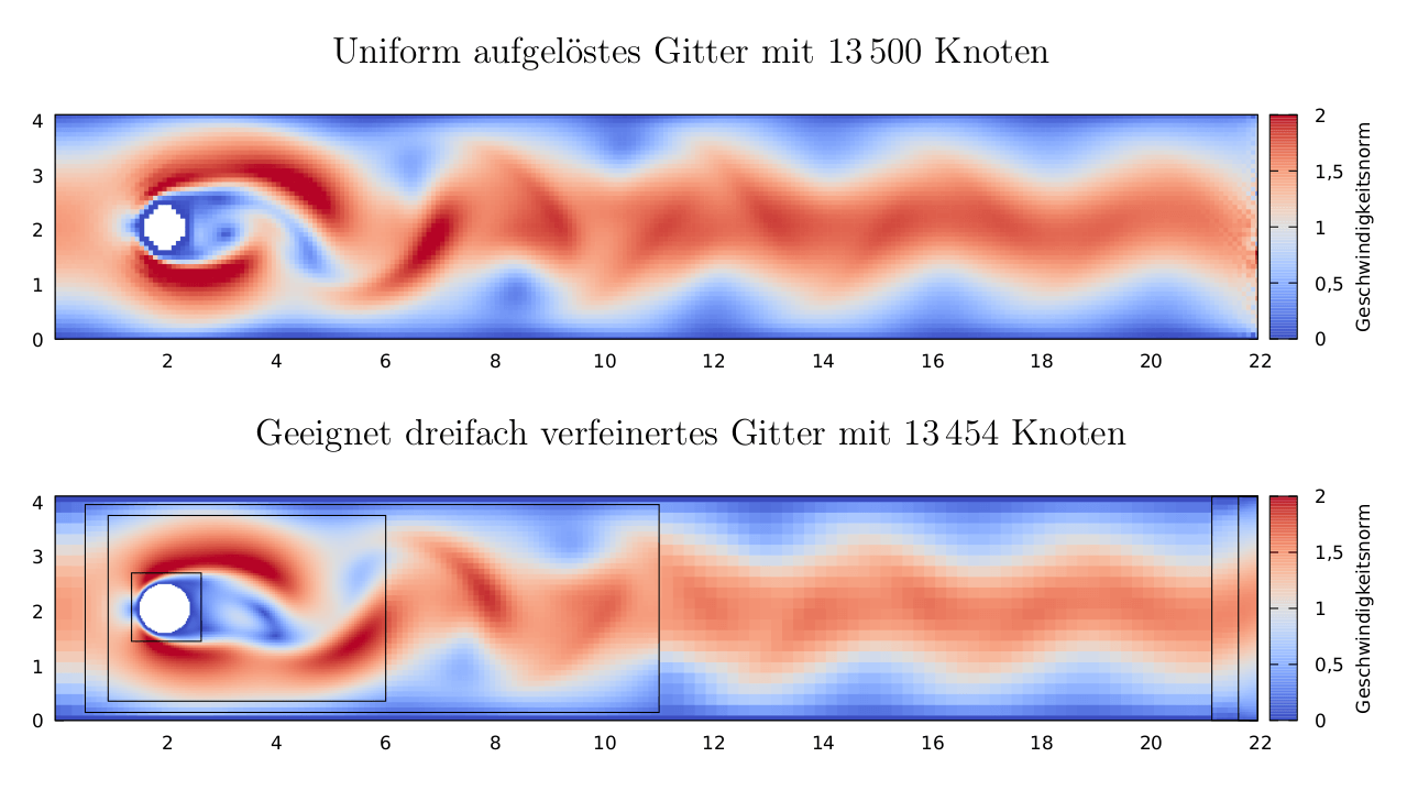
</p><video controls="" loop="true" poster="https://static.kummerlaender.eu/media/lbm_with_curl.poster.jpg" preload="metadata" style="max-width:100%">
<source src="https://static.kummerlaender.eu/media/lbm_with_curl.mp4" type="video/mp4"/>
</video></div></content></entry><entry><id>https://code.kummerlaender.eu/compustream/commit/?id=fc02e4c5f8c8bbb014449dc27d7b69992ad6043f</id><title>Add basic physical scaling and Knudsen quality criterion</title><link title="Add basic physical scaling and Knudsen quality criterion" rel="alternate" href="https://code.kummerlaender.eu/compustream/commit/?id=fc02e4c5f8c8bbb014449dc27d7b69992ad6043f"/><author><name>Adrian Kummerländer</name></author><updated>2019_04_16T22:45:00+02:00</updated><content type="xhtml"><div xmlns="http://www.w3.org/1999/xhtml"><p>The paper <a href="https://arxiv.org/abs/1507.06767">Automatic grid refinement criterion for lattice Boltzmann method</a> by Lagrava et al. describes a criterion for measuring the local simulation quality using a comparison of the theoretical Knudsen number and the quotient of the cells’s non-equilibrium and equilibrium function.</p><video controls="" loop="true" poster="https://static.kummerlaender.eu/media/compustream_quality_display.teaser.jpg" preload="metadata" style="max-width:100%">
<source src="https://static.kummerlaender.eu/media/compustream_quality_display.mp4" type="video/mp4"/>
</video><p>While this criterion was developed to enable automatic selection of areas to be refined, it also offers a interesting and unique perspective on the fluid structure.</p><p>As the criterion requires calculation of the modeled Reynolds-, Mach- and Knudsen-numbers I took the time to set up the basics for scaling the simulation to actually model a physical system. Or rather calculating which physical model is represented by the chosen resolution and relaxation time.</p></div></content></entry><entry><id>https://code.kummerlaender.eu/grid_refinement_bsc_thesis/commit/?id=e4ba166e0cc77d78e882126a97a9681f1de2bb20</id><title>Published my BSc thesis on grid refined LBM in OpenLB</title><link title="Published my BSc thesis on grid refined LBM in OpenLB" rel="alternate" href="https://code.kummerlaender.eu/grid_refinement_bsc_thesis/commit/?id=e4ba166e0cc77d78e882126a97a9681f1de2bb20"/><author><name>Adrian Kummerländer</name></author><updated>2019_03_26T20:23:00+02:00</updated><content type="xhtml"><div xmlns="http://www.w3.org/1999/xhtml"><p>In addition to the <a href="https://static.kummerlaender.eu/media/gitterverfeinerte_lbm_in_openlb.pdf">PDF</a> (German, ~60 pages) all sources including any referenced simulation data are available on <a href="https://github.com/KnairdA/grid_refinement_bsc_thesis/">Github</a> and <a href="https://code.kummerlaender.eu/grid_refinement_bsc_thesis">cgit</a>. The resulting actual implementation of the grid refinement method by <a href="https://dl.acm.org/citation.cfm?id=2222180">Lagrava et al.</a> in <a href="https://www.openlb.net/">OpenLB</a> is currently not available publicly and likely wont make it into the next release. Nevertheless – if you are interested in the code and I have not yet found the time to release a rebased patch for the latest OpenLB release don’t hesitate to <a href="https://tree.kummerlaender.eu/contact">contact me</a>.</p><p><img alt="Visual comparison between refined and unrefined flow around a cylinder" src="https://static.kummerlaender.eu/media/grid_refinement_teaser.png"/></p><p>As a side note: The gnuplot-based <a href="https://code.kummerlaender.eu/grid_refinement_bsc_thesis/tree/img/common">setup</a> for efficiently transforming <a href="https://www.paraview.org/">Paraview</a> CSV exports into plots such as the one above (i.e. plots that are neither misaligned Paraview screenshots nor overlarge PDF-reader-crashing PGFPlots figures) might be of interest even if one doesn’t care about grid refinement or Lattice Boltzmann Methods (which would be sad but to each their own :-)).</p></div></content></entry><entry><id>https://code.kummerlaender.eu/compustream/commit/?id=84666523e9a278ac95ca43dbaa534e8aaaf3ebd2</id><title>Compustream performance improvements and interactive wall drawing</title><link title="Compustream performance improvements and interactive wall drawing" rel="alternate" href="https://code.kummerlaender.eu/compustream/commit/?id=84666523e9a278ac95ca43dbaa534e8aaaf3ebd2"/><author><name>Adrian Kummerländer</name></author><updated>2019_02_25T22:08:00+02:00</updated><content type="xhtml"><div xmlns="http://www.w3.org/1999/xhtml"><p>I found some time to further develop my GLSL compute shader based interactive LBM fluid simulation previously described in <a href="https://blog.kummerlaender.eu/article/fun_with_compute_shaders_and_fluid_dynamics"><em>Fun with compute shaders and fluid dynamics</em></a>. Not only is it now possible to interactively draw bounce back walls into the running simulation but performance was greatly improved by one tiny line:</p><pre>glfwSwapInterval(0);
</pre><p>If this function is not called during GLFW window initialization the whole rendering loop is capped to 60 FPS – including compute shader dispatching. This embarrassing oversight on my part caused the simulation to run way slower than possible.</p><video controls="" loop="true" poster="https://static.kummerlaender.eu/media/compustream_with_walls.poster.jpg" preload="metadata" style="max-width:100%">
<source src="https://static.kummerlaender.eu/media/compustream_with_walls.mp4" type="video/mp4"/>
</video></div></content></entry><entry><id>https://code.kummerlaender.eu/nixos_system/commit/?id=55daf8a35f4f1761f5f4c4ebe4a6dcb4b0ace514</id><title>Describe custom gitolite and cgit setup</title><link title="Describe custom gitolite and cgit setup" rel="alternate" href="https://code.kummerlaender.eu/nixos_system/commit/?id=55daf8a35f4f1761f5f4c4ebe4a6dcb4b0ace514"/><author><name>Adrian Kummerländer</name></author><updated>2018_10_01T08:26:00+02:00</updated><content type="xhtml"><div xmlns="http://www.w3.org/1999/xhtml"><p>Replaces short-term Gitea instance on <code>code.kummerlaender.eu</code>.</p><p>The main reason for implementing this more complex setup is that Gitea both lacks in features in areas that I care about and provides distracting features in other areas that I do not use.</p><p>e.g. Gitea provides multi-user, discussion and organization support but doesn’t provide Atom feeds which are required for <a href="https://tree.kummerlaender.eu/projects/xslt/overview/">Overview</a>.</p><p>This is why exposing <a href="http://gitolite.com">gitolite</a>-managed repositories via <a href="https://git.zx2c4.com/cgit/about/">cgit</a> is a better fit for my usecases.</p><p>Note that gitolite is further configured outside of Nix through its own admin repository.</p><p>As a side benefit <code>pkgs.kummerlaender.eu</code> now provides further archive formats of its Nix expressions which simplifies Nix channel usage.</p></div></content></entry><entry><id>https://code.kummerlaender.eu/blog.kummerlaender.eu/commit/?id=c08fbb73a960bd19ab1ca553da5bb8111622baba</id><title>Nixify build process</title><link title="Nixify build process" rel="alternate" href="https://code.kummerlaender.eu/blog.kummerlaender.eu/commit/?id=c08fbb73a960bd19ab1ca553da5bb8111622baba"/><author><name>Adrian Kummerländer</name></author><updated>2018_06_04T21:12:00+02:00</updated><content type="xhtml"><div xmlns="http://www.w3.org/1999/xhtml"><p>Building the website in the presence of the Nix package manager is now as simple as:</p><ul>
<li>cloning this repo</li>
<li>entering the nix-shell environment declared by <code>shell.nix</code></li>
<li>calling <code>generate</code></li>
<li>optionally call <code>preview</code> to spawn a webserver in <code>target/99_result</code></li>
</ul><p>All dependencies such as the internal InputXSLT, StaticXSLT and BuildXSLT modules as well as external ones such as KaTeX and pandoc are built declaratively by Nix.</p></div></content></entry></feed>